MOS1.3. Excel Advanced (English)

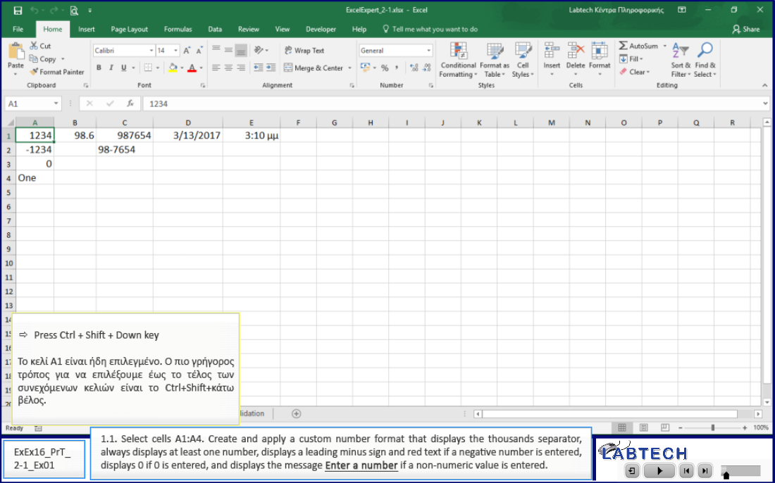
1. Open the ExcelExpert_2-1 workbook, display the Custom Data Formatting worksheet, and do the following:

1.1. Select cells A1:A4. Create and apply a custom number format that displays the thousands separator, always displays at least one number, displays a leading minus sign and red text if a negative number is entered, displays 0 if 0 is entered, and displays the message Enter a number if a non-numeric value is entered.

• Δείτε τη σελίδα Key για λεπτομερή επεξήγηση.

1.2. Select cell B1. Create and apply a custom number format that displays the thousands separator and the decimal point, always displays at least one digit before and after the decimal point, and displays °C (the degree symbol and the letter C, for degrees Celsius) at the end.

• Εδώ ζητείται μόνο μορφοποίηση των θετικών αριθμών που είναι ούτως ή άλλως στο πρώτο μέρος της σύνταξης, άρα δεν χρειάζεται να εισάγουμε διαχωριστικά για τα υπόλοιπα (τα παραλείπουμε).

1.3. Select cells C1:C2. Create and apply a custom number format that displays a six-digit entry with a dash after the first two digits, the text Acct # before the digits, and the text Enter numbers only if the user includes any non-numeric characters in the entry.

• Εδώ δεν αναφέρεται η μορφοποίηση που θα έχει το 0 άρα την παραλείπουμε.

1.4. Select cell D1. Create and apply a custom date format that displays the two-digit month, day, and year, separated by periods.

1.5. Select cell E1. Create and apply a custom time format that displays the two-digit hour and minute with nothing in between them, followed by a space and the text hours.

• • Δείτε τη σελίδα Key για τις σωστές custom μορφές - βέβαια μπορείτε να τα δείτε κι από το αρχείο αποτελέσματος επιλέγοντας κάθε φορά τα αντίστοιχα κελιά και εμφανίζοντας το π.δ. Format Cells > Custom.

ExEx16_PrT_2-1_Ex01

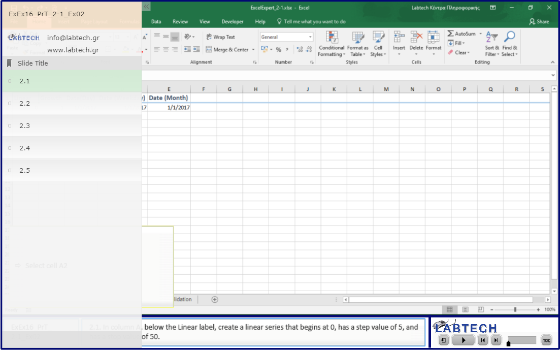
2. Display the Fill Series worksheet and do the following:

2.1. In column A, below the Linear label, create a linear series that begins at 0, has a step value of 5, and has a stop value of 50.

2.2. In column B, below the Growth label, create a growth series that begins at 1, has a step value of 2, and has a stop value of 250.

2.3. Fill the range C2:C11 with a Date series that uses a day unit and a step value of 2.

2.4. Fill the range D2:D11 with a Date series that uses a weekday unit and a step value of 1.

2.5. Fill the range E2:E11 with a Date series that uses a month unit and a step value of 6.

Σημείωση; 
Για να γίνει συμπλήρωση σειρών, πρέπει να υπάρχει αυτή η σειρά "περασμένη" στο Excel. Συνήθως οι μήνες και οι ημέρες υπάρχουν έτοιμοι. Για να βρείτε ποιες σειρές υπάρχουν στην εφαρμογή σας, ακολουθήστε τα βήματα: File > Options > Advanced > General section > Edit Custom Lists... button - στο π.δ. Custom Lists θα δείτε αν υπάρχει η σειρά των αγγλικών ή των ελληνικών μηνών / ημερών ή όχι - αν δεν υπάρχει μπορείτε να την προσθέσετε από το NEW LIST (δυστυχώς θα πρέπει να πληκτρολογήσετε όλη τη σειρά) ώστε να είναι διαθέσιμη για αυτόματη συμπλήρωση μελλοντικά.

ExEx16_PrT_2-1_Ex02

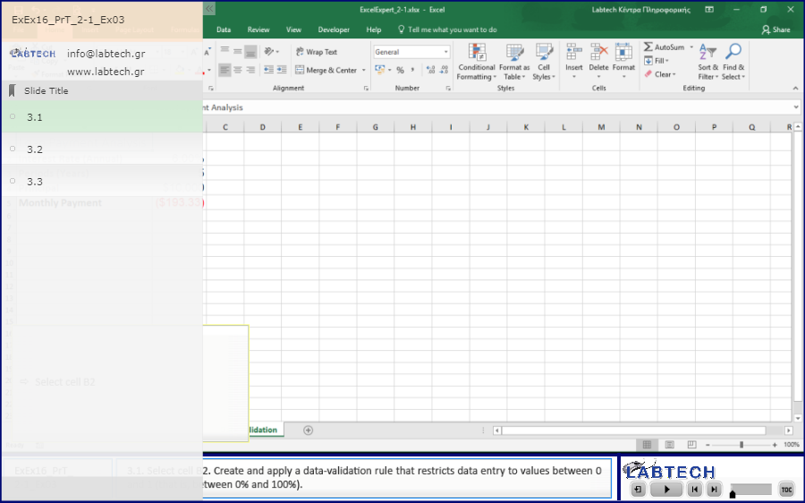
3. Display the Data Validation worksheet and do the following:

3.1. Select cell B2. Create and apply a data-validation rule that restricts data entry to values between 0 and 1 (that is, between 0% and 100%).

• • • Επιλέξτε μορφή Decimal (δεκαδική) από τη λίστα καθώς πρόκειται για ποσοστά.

3.2. Include an input message titled Interest Rate with the following text: Please enter a value between 0 and 1.

3.3. Then enter a stop-style error message titled Invalid Interest Rate with the following text: The interest rate value you entered is invalid. Please enter a value between 0 and 1.

3.4. Select cell B3. Create and apply a data-validation rule that restricts data entry to positive values with a minimum of 1 and a maximum of 30.

• • • Εδώ πρόκειται για χρονική περίοδο σε έτη οπότε μπορείτε να επιλέξετε Whole number (ακέραιο).

3.5. Include an input message titled Loan Period with the following text: Please enter a value between 1 and 30 years.

3.6. Then enter a stop-style error message titled Invalid Loan Period with the following text: The loan period value you entered is invalid. Please enter a value between 1 and 30 years.

3.7. Select cell B4. Create and apply a data-validation rule that restricts data entry to positive values.

• • • Εδώ πρόκειται για το κεφάλαιο (Principal) οπότε επίσης θα επιλέξουμε ακέραιους αριθμούς.
    • Από τη λίστα Data επιλέξτε greater than (μεγαλύτερο από).

3.8. Include an input message titled Loan Principal with the following text: Please enter a value greater than 0. 

3.9. Enter a stop-style error message titled Invalid Loan Principal with the following text:  The loan principal value you entered is invalid. Please enter a value greater than 0.

ExEx16_PrT_2-1_Ex03

4. Save the workbook.

5. Open the ExcelExpert_2-1_results workbook. Compare the two workbooks to check your work. Then close the open workbooks.

On the "Product Inventory" worksheet, format column B to display numeric values to two decimal places. The format should be applied to existing and new rows.

• Θα πρέπει να επιλεχθεί ολόκληρη η στήλη ώστε να εφαρμοστεί η μορφή τόσο στις υπάρχουσες όσο και στις νέες γραμμές.

On the "Accounts Receivable Data" worksheet, format column F so that any time value entered in the column is displayed as "mm/yy". The days should not be displayed.

• Είναι καλή πρακτική να εντοπίσετε την πλησιέστερη μορφή σε αυτήν που ζητά η άσκηση, και να την τροποποιήσετε.

On the "ProjectDatabase" worksheet, using the Fill Series option in Excel, fill in the Projects May through November in cells D3:I3. Do not change the cell formatting.

• Αν η συμπλήρωση δεν γίνεται σε πίνακα αλλά σε απλά κελιά, θα χρειαστεί αντί για Fill Series να επιλεχθεί από το κουμπί AutoFill Options το Fill Without Formatting.
• Αν η συμπλήρωση των μηνών δεν είναι εφικτή στον υπολογιστή σας, λογικά δεν υπάρχει η συγκεκριμένη λίστα. Μπορείτε να τη δημιουργήσετε (File > Options > Advanced > ομάδα General, κουμπί Edit Custom Lists... ) ή να δοκιμάσετε με τους μήνες στα Ελληνικά αν θέλετε απλώς να δείτε τη διαδικασία. 

On the "Student Grades" worksheet, add data validation to cells C3:C48 that displays a Stop error with the title "Not valid" and the text " 1 to 100" when the user enters a value less than 1 or greater than 100 or a number that includes a decimal digit.

• Δεν επιτρέπονται τιμές <1 ή >100, άρα θα επιτρέπονται τιμές >=1 και <=100, δηλαδή between (minimum) 1 and (maximum) 100. 
• Επιλέγουμε Whole numbers only ώστε να μην επιτρέπεται η εισαγωγή δεκαδικών αριθμών (decimal digits).